Validate Data Mining In Tableau With A Chi-Square Test

I have just enrolled in a Data Science course on Udemy  and I learned good stuff.

In this article we will start using statistics. Don’t worry we’ll do something simple, we’ll use the Chi-square test in a basic way. There is a special section to learn how to do statistics at an advanced level.

I’ll explain why we’re going to learn how to use the Chi-square test. The results we have with theses 2 bar charts are good. We see on theses 2 bar charts that age has a significant impact on the rate of client leaving the bank. We also see in which age groups the clients leaves the bank the most and which age groups the clients leave the bank the least. With that we have good insights.

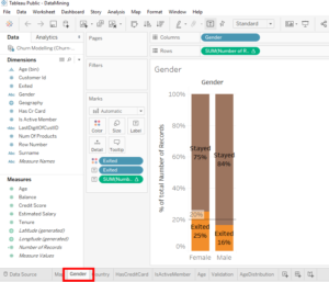
In the A/B test « Gender », we can see that there is a correlation between the male and female sex and the choice to leave the bank. But as I said before, this A/B test is basic. The results of a basic A/B test visually shows us what is probably happenning in reality but we aren’t 100% sure of these results. To validate these results, we need do to use statistical tests like Chi-square test.

Doing a report based on basic A/B test is very risky and you can have completely false insights. I don’t advise you to do it (unless you want to leave your job). It’s for this reason that using Chi-square will help us to have strong insights.

Chi-square will allow us to know if our results are statistically significant. Our results are based on a sample of 10 000 clients and Chi-square test will tell us if these results are due to chance effects or if these results can represent all the client of the bank.

For example in our A/B test « Gender », we observed that in our sample of 10 000 clients, women are more likely to leave the bank compared to men.

Now, we aren’t sure if the results of this sample represent the behavior of all the bank’s clients.

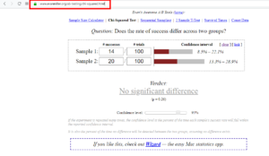
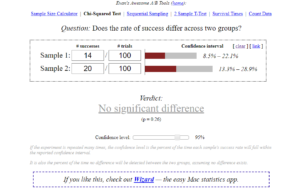
To use basic Chi-square test, we use an online tool. Click here  .

On internet, there are plenty of websites to do a Chi-square test but we’ll use this one so that you can understand how it works. To do a Chi-square test, we need to use absolute values and in our A/B test we have percentage.

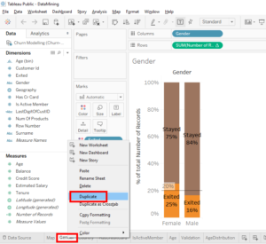
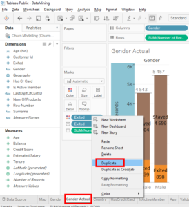
Let’s go back to Tableau. We’ll create a new tab with a version of A/B test with absolute values. In this way, we keep the A/B test with the percentages. Do a right-click on the « Gender » tab and select « Duplicate ».

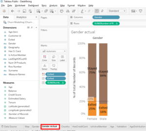
Name the new tab « Gender Actual » to specify that it’s absolute values.

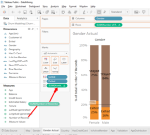
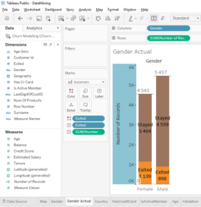
To have the absolute values, move « Number of Records » in « Measures » to the « Marks » area and put it over top of « SUM(Number of Records ».

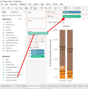
Move « Number of Records » in « Measures » to « Rows » over « SUM(Number of Records ».

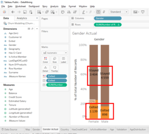
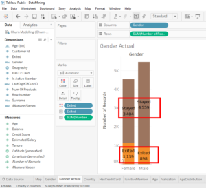
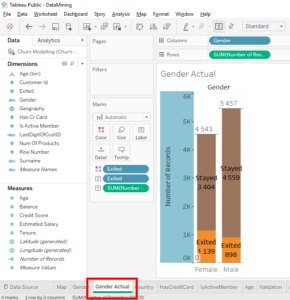
Cool, we have our absolute values.

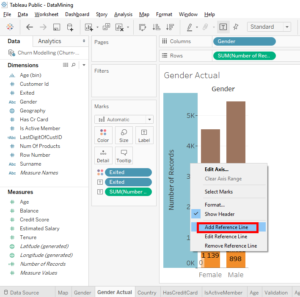
We also need total absolute values, which means the total number of men and women. There is a very fast way to get that. Right-click on the vertical axis and select « Add Reference Line ».

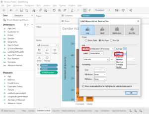
Then in « Value », click on the drop-down on the right and select « Sum » to have the total sum of the observations.

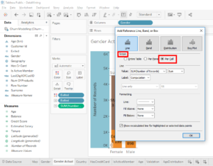
And in « Scope », you select « Per Cell » option to specify that you want the total sums for each category, male and female.

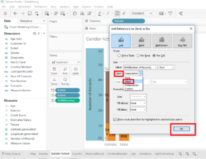
Now, we have the total sum at the top of the bars. We will modify labels to have the absolute values. In « Label », we will change « Computation » to « Value » and click on the « OK » button.

Perfect, we have the total amount of observation at the top of each bar : 4543 women and 5457 men. We have what we need to use our online tool.

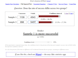
OK, I’ll explain how this tool works. « Sample1 » and « Sample2 » correspond to the independent variable « Gender ». You choose in which order you enter the data, « Sample1 » for men or the opposite. In our case, we use « Sample1 » for women and « Sample2 » for men.

« #success » corresponds to the result Y=1, which means in our case « yes, the client left the bank ».

« #trials » is the total number of observations, which means the total number of women in « Sample1 » and the total number of men « Sample2 ».

That’s how you enter the data :

• For « Sample1 » in #success, you enter 1139 because there are 1139 women who left the bank. For « Sample1 » in #trials, you enter 4543 because there are 4543 women in total.

 

• For « Sample2 » in #success, you enter 898 because there are 898 men who left the bank. For « Sample2 » in #trials, you enter 5457 because there are 5457 men in total.

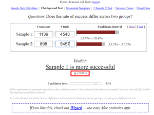
Here is the verdict : « Sample1 is more successful ». « Sample1 » corresponds to women and #success is :« yes, the client left the bank ». This verdict means that of all the bank’s client, women are more likely to leave the bank than men. And look, there is something important, it’s « p<0.001 ». This means that the « p » is strictly less than 0.001.

« p » is the value that indicates whether an independent variable has a statistically significant effect on a dependent variable. In our case, the independent variable is « Gender » and the dependent variable is « Exited », which is : « yes, the client left the bank ». So « p » is strictly less than 0.001, which means that the independent variable « Gender » has a statistically significant effect on the dependent variable « Exited ». This shows us that out of the total number of bank’s clients, women are more likely to leave the bank than men.

This is how we use Chi-square test with this online tool. This is the same principle on all online tools that you can find on Google or DuckDuckGo . You can repeat these instructions that I gave you with other tools, you will get the same results.

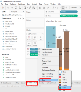
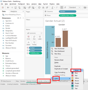
It’s cool with the Chi-square we validated the A/B test and to specify that this A/B test is validated, we’ll color the tab in green.

Right-click on the tab, select « Color » and select « Green ».

Perfect, now we’ll validate another A/B test. Selects « HasCreditCard » tab.

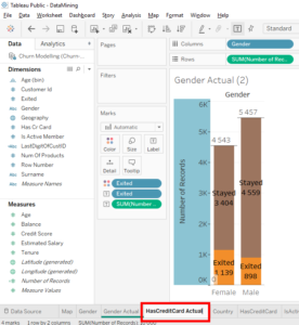
We’re going to create an A/B test « HasCreditCard » only with absolute values. To save time, right-click on « Gender Actual » tab and select « Duplicate ».

We’ll remove the green color on the tab « Gender Actual (2) ». Right-click on the tab and select « Color » and « None ».

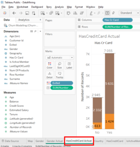
You rename the tab « HasCreditCard Actual ».

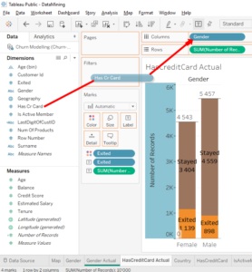
Move the variable « HasCrCard » over « Gender » in « Columns ».

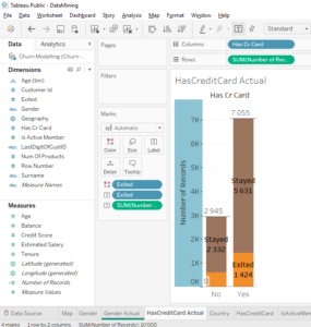
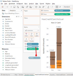
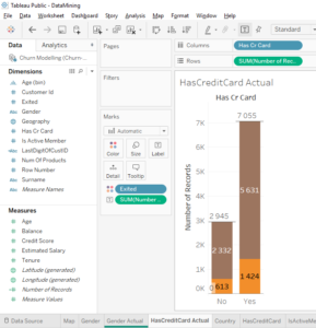
Excellent, everything is ready to do a Chi-square test. We’ll remove « Exited » labels to better see the absolutes values. Make a click and drag out.

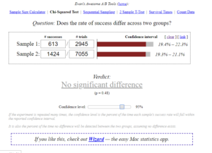
Perfect, let’s go back to our online tool. In this case, « Sample1 » is « no », which means client who don’t have credit card and « Sample2 » for « yes », which means clients who have a credit card.

That’s how you enter the data :

• For « Sample1 » in #success, you enter 613 because there are 613 clients who left the bank. For « Sample1 » in #trials, you enter 2945 because there are 2945 clients who don’t have a credit card.

• For « Sample2 » in #success, you enter 1424 because there are 1424 clients who left the bank. For « Sample2 » in #trials, you enter 7055 because there are 7055 clients who have a credit card.

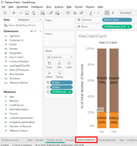
Let’s look at the verdict, it’s « No significant difference ». « p » value is very high, it’s above 5%. This confirms that the independent variable « HasCrCard » has no statistically significant effect on the dependent variable « Exited ». That was the conclusion we had made when we had done the A/B test with percentages.

We had seen that there was 21% of « Exited » (clients who left the bank) in the category « no » and 20% in the category « yes ». With these results we concluded that most likely the variable « HasCrCard » had no impact on the rate of clients who left the bank. Chi-square test confirms our conclusion and we can put the tab « HasCrCard » in green to say that it’s OK.

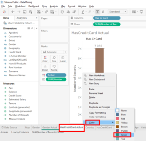
Right-click on the tab « HasCreditCard » => « Color » => « Green ».

Excellent, now, you can do a statistical A/B test with 2 categories. Soon, we will do statistical A/B tests with more than 2 categories.

Share this article if you think it can help someone you know. Thank you.

-Steph